Which credit card should we offer?
FiTech · Credit-card offer design and campaign optimization
A product that attracts the most applicants is not automatically the product that creates the most value. FiTech’s credit-card case makes that tension concrete: lower interest and no annual fee can raise response while reducing the value of each acquired customer.
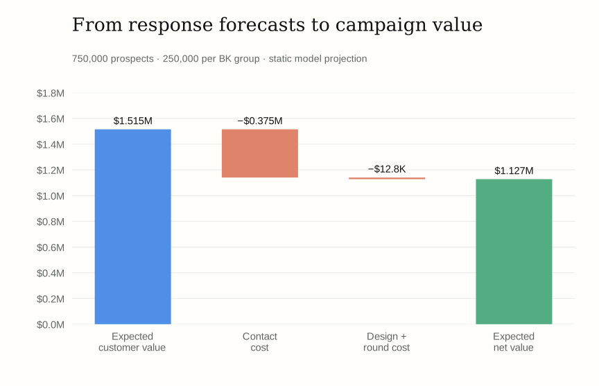
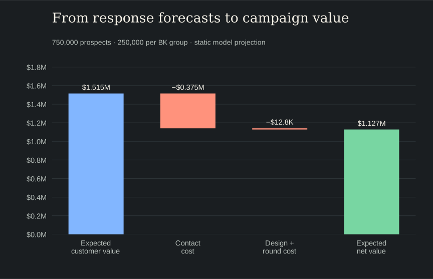
The analysis combines a response model with the case’s customer lifetime values, then chooses an offer for each of three BK score groups under campaign-cost constraints. The reproduced static plan generates $1.127M in expected net value, approximately $111,808 more than the best single-offer plan. Both amounts are model projections for the case.
Start with the economics of a response
The source workbook contains 14 historical campaign cells, representing 1,520,000 contacts and 27,486 responses, plus 12 proposed products with CLV values for BK groups 150, 200, and 250. The score labels are treated as the case’s segments; they are not mapped to an external credit-rating scale.
The proposed products vary APR, fixed versus variable rates, and annual fees. Under the notebook’s customer-preference assumptions—lower APR, lower fees, and a fixed rate preferred—offer 3 is the most attractive: 14.9% fixed APR with no annual fee.
But its supplied CLV falls from $52 in BK 150 to $2 in BK 250. Maximizing responses to that offer across all segments would ignore a substantial change in acquisition economics.
Estimate response without expanding 1.52 million rows
The source notebook represents each historical cell as opened and not-opened rows, weighted by their counts. The reproduction uses the equivalent grouped binomial likelihood, retaining those counts without constructing a row for every contact:
model = smf.glm(
    "response_rate ~ apr + annual_fee + bk_score + C(fixed_var)",
    data=hist,
    family=sm.families.Binomial(),
    freq_weights=hist.nr_emailed,
).fit()
This is the adapted reproduction code. The weights matter: a cell representing 200,000 contacts should contribute more information than one representing 10,000. The predictors follow the original response model.
The fitted APR coefficient is about −0.271: a one-percentage-point increase in APR is associated with an odds multiplier of approximately 0.763, holding the included variables fixed. The variable-rate indicator also lowers predicted response relative to fixed rates. These are model associations from a small set of campaign cells; campaign timing and other omitted differences could affect them.
Translate predictions into an offer decision
For each of the 36 offer–segment combinations, the analysis calculates expected customer value and subtracts the $0.50 contact cost:
score_rows.append(
    s.with_columns((pl.col("p_open") * pl.col("clv")).alias("ev_per_email"))
)
score_table = pl.concat(score_rows).with_columns(
    (pl.col("ev_per_email") - 0.5).alias("margin_per_email")
)
This excerpt follows the source notebook’s scoring calculation, with formatting adjusted. It creates a common economic scale for comparing products, rather than treating response probability as the objective.
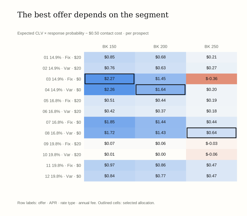
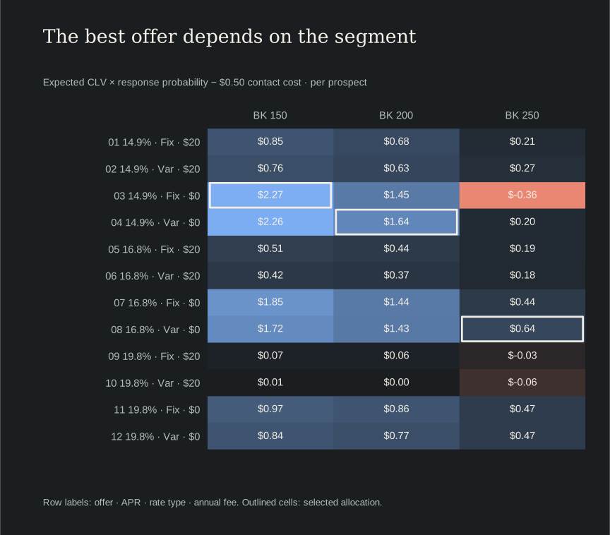
The most revealing comparison is in BK 250. Offer 3 has the highest predicted response, approximately 6.97%, but only $2 CLV. Its expected margin is therefore about −$0.36 per prospect. Offer 8 has a lower predicted response of 3.57%, yet its $32 CLV yields approximately +$0.64 per prospect.
The response leader would lose money under these assumptions. The value calculation changes the decision.
Account for the cost of using more products
The case allocates 250,000 prospects to each BK group, for 750,000 total contacts. It also charges $800 per round, $10,000 for the first solicitation design, and $1,000 for each additional design.
With 12 candidate offers, there are only 4,095 nonempty offer subsets. Exhaustive enumeration is practical: for each subset, assign each segment its highest-margin available offer, deduct the design and round costs, and retain the best plan.
pick = {
    bk: max(subset, key=lambda offer: margin[(offer, bk)])
    for bk in bk_levels
}
gross_margin = sum(BK_QUOTA * margin[(pick[bk], bk)] for bk in bk_levels)
net = gross_margin - fixed_cost(len(subset))
This is the core source optimization step, reformatted for readability. Once a subset is fixed, the objective is linear within a segment, so its quota goes to that segment’s best available offer. Enumerating subsets then handles the shared design costs.
| Segment | Selected offer | Product | Contacts |
|---|---|---|---|
| BK 150 | 3 | 14.9% fixed, $0 annual fee | 250,000 |
| BK 200 | 4 | 14.9% variable, $0 annual fee | 250,000 |
| BK 250 | 8 | 16.8% variable, $0 annual fee | 250,000 |
The best single-offer solution sends offer 4 to everyone and produces approximately $1.016M in expected net value. Segment-specific selection increases that to $1.127M, a projected 11.0% gain after the extra design costs.
What should happen before a rollout?
The static optimizer is exact for its inputs, but the response estimates are uncertain. Fourteen campaign cells provide limited coverage of the offer space, even though their contact counts are large. The fitted model is not an independent validation of all 36 proposed combinations.
The original notebook also lays out a two-round test-and-learn extension. No Round 1 feedback file was present in the supplied repository, so this page reports the reproducible static plan rather than presenting an updated second-round result as observed.
A useful next experiment would test the most competitive offers within each BK group, update response estimates, and check whether the extra segmentation value persists. It should also revisit the CLV assumptions: if the value of newly acquired customers changes, a formerly attractive offer can become unprofitable even when its response rate stays high.
Reproduction notes
This is a UC San Diego Rady course case, reproduced from fitech.ipynb in mgta455-fitech-Group-6 (source snapshot 90da042). Figures were regenerated from the supplied data; amounts described as expected or projected are model outputs, not realized company results.
The grouped binomial refit reproduces the saved notebook coefficients and the $1,127,461.47 expected-net-value result. All 4,095 offer subsets are enumerated, and segment allocations sum to 750,000. The direct grouped calculation replaces a memory-heavy row expansion; the original offer definitions, CLVs, quotas, and costs are preserved.
The reproduction exports aggregate results only. The data files remain in the original course repository. The downloadable script accepts a local repository path; it does not require the original Docker environment. The website itself uses the generated SVGs and does not retrain models during a build.
Aggregate results · Reproduction code · Figure code · Environment requirements