Choose the next product by value
Pentathlon · Next-product recommendations using expected contribution
An email recommendation has at least two ways to look successful: it can generate a purchase, or it can generate a valuable purchase. Pentathlon’s next-product case asks how the recommendation changes when both matter.
The reproduced analysis finds that maximizing expected contribution changes the recommended option for 56.7% of held-out customers compared with maximizing response probability. Its projected contribution is 12.4% above the best uniform message and 8.5% above response-only targeting, before contact costs.
Define the decision before fitting the model
The dataset contains 600,000 customer observations across six department messages—endurance, strength, water, team, backcountry, and racquet—and a no-message control. The supplied split has 420,000 training observations and 180,000 test observations.
The outcomes are whether a customer purchased within the response window and the total order value across departments, conditional on purchasing. Historical department-level purchase frequency, age, and other customer or neighborhood characteristics form the predictors. The neighborhood variables describe an area; they should not be read as exact individual characteristics.
The business decision is to select one of the seven options for each customer. Retaining no message as a valid choice gives the policy a way to avoid sending an email when its modeled alternative is better.
Two models answer two different questions
First, a logistic model estimates purchase probability for each possible message. Second, a linear model fitted to the 10,080 training buyers estimates order value conditional on a purchase. The source interacts every predictor with the message, allowing different relationships across departments.
ivar = [f"{e}:message" for e in evar if e != "message"]

clf_int = rsm.model.logistic(
    data={"pentathlon_nptb": pentathlon_nptb.filter(pl.col("training") == 1)},
    rvar="buyer", lev="yes", evar=evar, ivar=ivar,
)
This excerpt condenses the original interaction-model setup. A customer’s purchase history can matter differently for a racquet promotion than for an endurance promotion. The order-value model uses the same predictor structure, fitted only to purchasers.
The reproduction fits equivalent separate models by message, which avoids constructing a much larger interaction matrix. It estimates the same response and conditional-order relationships, then scores every held-out customer under every option. Response AUC within the actually received message groups ranges from 0.858 to 0.897; this checks purchase ranking, not the value of assigning a different message.
Choose the message using expected contribution
The case assumes a 40% gross margin. For each customer and message, expected contribution is purchase probability multiplied by conditional order value and margin:
margin = 1 - 0.60
pentathlon_nptb = pentathlon_nptb.with_columns(
    **{
        f"ep_{m}": pl.col(f"p_{m}") * pl.col(f"total_os_{m}") * margin
        for m in msg_levels
    }
)
These lines reproduce the source scoring rule. Conditional order predictions are clipped at zero, as in the notebook. The next step chooses the option with the highest expected contribution, rather than the highest purchase probability.
A simple illustration explains why the distinction matters: a 5% chance of a €20 order implies €0.40 contribution at a 40% margin. A 3% chance of a €50 order implies €0.60. These are illustrative numbers; the lower-response option is more valuable under the stated assumptions.
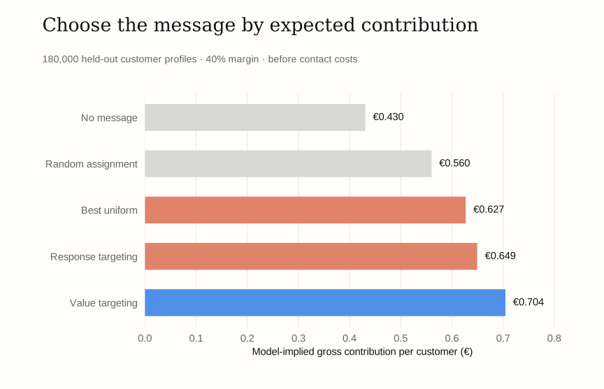
Value targeting produces approximately €0.704 per customer, versus €0.627 for sending endurance to everyone. The difference is €0.0776 per customer. Applied to the notebook’s five-million-customer campaign scenario, that implies approximately €387,795 additional gross contribution before contact costs.
The comparison with response targeting is also useful: its €0.649 estimate is better than the uniform baseline, yet still below the value-targeting estimate. Personalization and the choice of optimization objective each contribute to the forecast improvement.
The objective materially changes the allocation
Response targeting sends 69.9% of customers to endurance and 20.3% to strength. Value targeting reduces those shares to 40.8% and 4.6%, respectively, while increasing backcountry, team, racquet, and water recommendations.
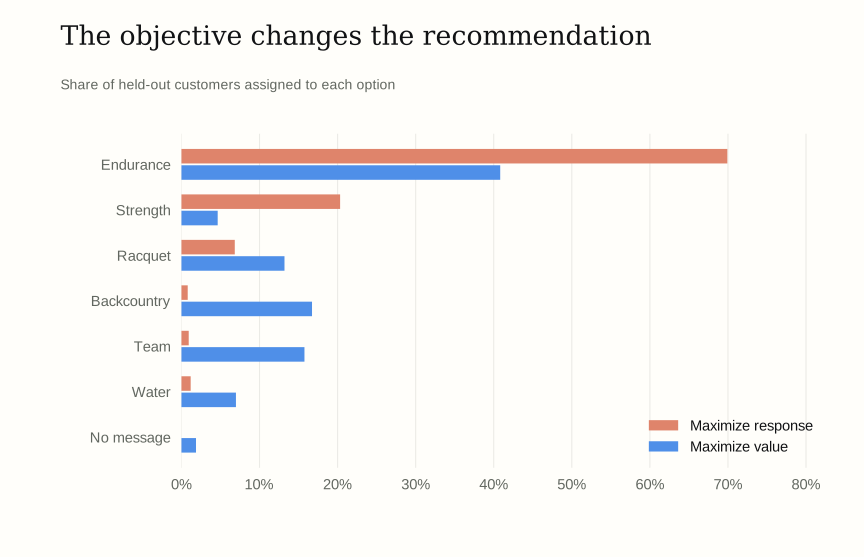
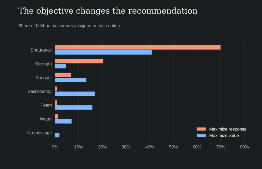
Overall, 56.7% of customers change recommendation when the objective switches from purchase probability to expected contribution. This is a substantial operating change: departments would see a different distribution of promotional exposure even though the underlying customer data stayed the same.
The no-message option is selected for 1.9% of customers by value targeting and for none by response targeting in this run. That result comes from the model’s comparison of purchase chance and basket value; it is not an unsubscribe or contact-fatigue model.
Separate a forecast from a policy test
The train/test separation protects model fitting from the held-out outcomes. But averaging predicted contribution over held-out features is still a model-based policy valuation. It does not observe what every customer would have spent under each alternative message. The predicted maximum can look attractive partly because the decision rule chooses the largest of several uncertain estimates.
The case also excludes contact costs from the contribution formula. Repeated messages could change fatigue, unsubscribe behavior, and future purchasing, none of which is captured by a single response-window calculation.
A practical next step is a randomized comparison of the value policy, the response policy, and the best uniform message, with a no-message holdout. The primary outcome should be contribution net of contact costs, accompanied by unsubscribe and longer-term customer-value measures. That would test whether the forecast improvement survives deployment.
Reproduction notes
This is a UC San Diego Rady course case, reproduced from pentathlon_nptb.ipynb in mgta455-pentathlon-nptb-Group-6 (source snapshot 006097f). Figures were regenerated from the supplied data; amounts described as expected or projected are model outputs, not realized company results.
The separate message-specific logistic and conditional OLS fits reproduce the original fully interacted models: expected contribution is €0.704499 for value targeting and €0.626940 for the uniform endurance message. Best-uniform selection uses training predictions; the original notebook selects it on held-out predictions, with the same winner here. The random baseline retains seed 455. This article focuses on the interpretable two-stage analysis rather than the later neural-network, random-forest, and boosted-model search.
The reproduction exports aggregate results only. The data files remain in the original course repository. The downloadable script accepts a local repository path; it does not require the original Docker environment. The website itself uses the generated SVGs and does not retrain models during a build.
Aggregate results · Reproduction code · Figure code · Environment requirements