demo_pi_A <- 0.22
demo_pi_B <- 0.18
demo_n <- 1000

demo_cta_a <- rbinom(demo_n, size = 1, prob = demo_pi_A)
demo_cta_b <- rbinom(demo_n, size = 1, prob = demo_pi_B)A/B Testing a Call to Action
Simulating Key Ideas from Classical Frequentist Statistics
A simulation-based walkthrough of A/B testing, uncertainty, and hypothesis testing using a simple homepage CTA experiment.
Introduction
Suppose I run a website with a landing page that invites visitors to join an email newsletter. The page has a prominent call to action, and I want to know whether slightly different wording changes how often visitors actually sign up.
For this post I will compare two versions of that CTA. Version A says Sign up for our newsletter here!, while version B says Stay up to date by signing up!. An A/B test assigns visitors at random to see one of the two messages, then compares the sign-up rates across groups. That random assignment is what makes the comparison meaningful: in expectation, the two groups differ only in the CTA they saw.
This business question turns out to be a nice way to illustrate several core ideas from classical frequentist statistics. Using simulated data, I will walk through estimation, uncertainty, the Law of Large Numbers, the bootstrap, the Central Limit Theorem, hypothesis testing, and one practical pitfall that often shows up in real experiments: peeking too early.
The A/B Test as a Statistical Problem
For each visitor, the outcome is binary: either they sign up for the newsletter or they do not. That makes a Bernoulli model a natural starting point. If a visitor sees CTA A, let their sign-up probability be \(\pi_A\); if they see CTA B, let it be \(\pi_B\).
The parameter I care about is the difference in conversion rates:
\[ \theta = \pi_A - \pi_B \]
If \(\theta > 0\), CTA A performs better. If \(\theta < 0\), CTA B performs better. If \(\theta = 0\), then the two messages are equally effective.
In practice I do not observe \(\pi_A\) and \(\pi_B\) directly. I only see sample outcomes, so I estimate the difference using the difference in sample means:
\[ \hat\theta = \bar{X}_A - \bar{X}_B \]
Because each observation is either 0 or 1, each sample mean is just a sample proportion. In other words, \(\bar{X}_A = \hat\pi_A\) and \(\bar{X}_B = \hat\pi_B\). This is one reason A/B tests are so intuitive: the estimator is simply the observed gap in conversion rates.
Simulating Data
In a real experiment I would not know the true conversion rates ahead of time. For a simulation exercise, though, setting the truth ourselves is exactly the point because it lets us evaluate how well our methods recover the answer. I will assume that CTA A has a true sign-up probability of 22.0% and CTA B has a true sign-up probability of 18.0%, so the true treatment effect is 0.040.
The code below simulates 1,000 Bernoulli outcomes for each CTA:
In this particular simulated sample, CTA A generated 225 sign-ups out of 1000 visitors, while CTA B generated 182 sign-ups. The observed difference in sign-up rates is 0.043, which is close to the true effect of 0.040.
| Observed Outcomes in the Simulated Experiment | |||
| Each CTA is shown to 1,000 visitors | |||
| CTA | Visitors | Sign-Ups | Observed Sign-Up Rate |
|---|---|---|---|
| CTA A | 1,000 | 225 | 22.5% |
| CTA B | 1,000 | 182 | 18.2% |
| True difference in sign-up rates: 0.040. Observed difference: 0.043. | |||
The Law of Large Numbers
The Law of Large Numbers says that as the sample size grows, the sample mean converges to the population mean. In the A/B testing setting, that matters because \(\hat\theta = \bar{X}_A - \bar{X}_B\) is built from sample averages. If we observe enough visitors, we should expect our estimate to stabilize near the true treatment effect.
To make that idea concrete, I pair the simulated A and B observations, compute the element-wise differences, and then track the running mean of those differences from 1 observation up through all 1,000 observations.
paired_diff <- cta_a - cta_b

lln_df <- tibble(
  n = 1:n_visitors,
  running_mean = cumsum(paired_diff) / n
)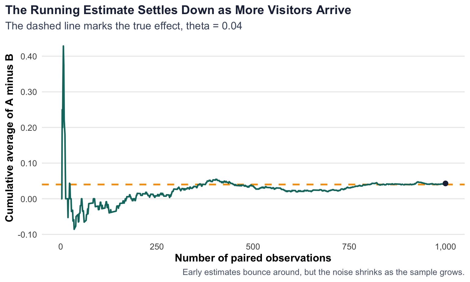
At the beginning of the plot, each new observation can move the estimate quite a bit. That is what sampling noise looks like when the sample is tiny. Later on, the line smooths out and stays much closer to the truth. By the end of the sample, the running estimate is 0.043, which is very close to the true difference of 0.040.
The main takeaway is not that the estimate becomes perfect, but that it becomes reliable. The Law of Large Numbers gives us a reason to trust large samples more than small ones.
Bootstrap Standard Errors
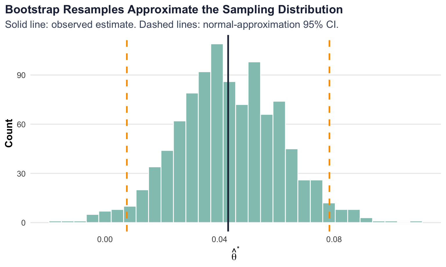
A point estimate tells me where the effect appears to be, but not how uncertain that estimate is. To quantify precision, I need a standard error. The bootstrap offers a practical way to get one: repeatedly resample from the observed data with replacement, recompute the statistic each time, and then look at how much those resampled estimates vary.
In this case, each bootstrap replication draws 1,000 outcomes with replacement from CTA A and 1,000 outcomes with replacement from CTA B, then computes a new difference in means \(\hat\theta^*\). Repeating that process many times gives an empirical approximation to the sampling variability of \(\hat\theta\).
Show bootstrap code
set.seed(496)

boot_estimates <- replicate(
  1000,
  mean(sample(cta_a, replace = TRUE)) - mean(sample(cta_b, replace = TRUE))
)

boot_se <- sd(boot_estimates)
ci_bounds <- theta_hat + c(-1.96, 1.96) * boot_se
For comparison, the analytical standard error for two independent Bernoulli samples is
\[ SE(\hat\theta) = \sqrt{\frac{\hat\pi_A(1 - \hat\pi_A)}{n_A} + \frac{\hat\pi_B(1 - \hat\pi_B)}{n_B}} \]
Using the observed sample proportions, the analytical standard error is 0.0180. The bootstrap standard error is 0.0180, which is very close. That is exactly what I would hope to see: the bootstrap is recovering essentially the same uncertainty estimate as the closed-form formula.
| Uncertainty Around the Estimated Treatment Effect | |
| Quantity | Value |
|---|---|
| Observed estimate | 0.0430 |
| Bootstrap standard error | 0.0180 |
| Analytical standard error | 0.0180 |
| 95% CI lower bound | 0.0076 |
| 95% CI upper bound | 0.0784 |
Using the bootstrap standard error, the resulting 95% confidence interval is [0.008, 0.078]. A careful frequentist interpretation is that if I were to repeat this full experiment many times and construct intervals the same way each time, about 95% of those intervals would cover the true effect. In this sample, the interval suggests that values near zero are less plausible than a modest positive lift for CTA A.
The Central Limit Theorem
The Central Limit Theorem says that the sampling distribution of the sample mean becomes approximately Normal as the sample size grows, even when the underlying data are not Normal. That matters here because our outcomes are Bernoulli, not bell-shaped. Even so, the difference in sample means can still behave approximately like a Normal random variable once the sample is large enough.
To show that visually, I simulate the estimator \(\hat\theta\) 1,000 times for each of four sample sizes: 25, 50, 100, and 500 visitors per group.
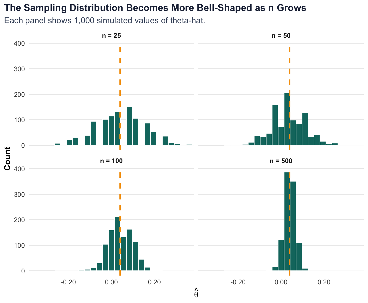
At n = 25, the histogram is jagged and clearly affected by discreteness. By n = 100, the shape is already noticeably smoother. At n = 500, the distribution looks much more symmetric and bell-shaped around the true effect. That is the CLT in action: even though individual observations are only zeros and ones, the estimator behaves increasingly like a Normal random variable as the sample size increases.
Hypothesis Testing
Once the CLT tells me that \(\hat\theta\) is approximately Normal in large samples, I can use that fact to perform a hypothesis test. The null hypothesis is
\[ H_0: \theta = 0 \]
and the alternative is
\[ H_1: \theta \neq 0 \]
The question is whether the observed data are surprising enough under the null that I am willing to reject it.
To answer that, I standardize the estimate:
\[ z = \frac{\hat\theta - 0}{SE(\hat\theta)} \]
The logic works step by step:
- By the CLT, \(\hat\theta\) is approximately Normal when the sample is large.
- Under the null, that distribution is centered at 0.
- Dividing by the standard error converts the statistic to something that is approximately standard Normal, which lets me compute a p-value.
This procedure is often described informally as a two-sample t-test, but in this Bernoulli setting it is more accurate to think of it as a large-sample z-test. The classical t-distribution result relies on Normal outcomes and estimated variance. Here the outcomes are not Normal, so the CLT is doing the heavy lifting.
| Hypothesis Test for Equal Sign-Up Rates | |
| Statistic | Value |
|---|---|
| Estimated effect | 0.0430 |
| Standard error | 0.0180 |
| z-statistic | 2.3917 |
| Two-sided p-value | 0.0168 |
For this simulated experiment, the test statistic is 2.392 and the p-value is 0.017. Because the p-value is below 0.05, I would reject the null of equal conversion rates at the 5% significance level. In plain language, this sample provides evidence that CTA A outperforms CTA B, with an estimated lift of about 4.3% in sign-up probability.
The T-Test as a Regression
The same comparison can be written as a simple linear regression. Stack the two groups into one dataset, define \(Y_i\) as the sign-up indicator, and let \(D_i = 1\) if visitor \(i\) saw CTA A and \(D_i = 0\) if they saw CTA B. Then estimate
\[ Y_i = \beta_0 + \beta_1 D_i + \varepsilon_i \]
This model is easy to interpret:
- \(\beta_0\) is the mean outcome for CTA B.
- \(\beta_0 + \beta_1\) is the mean outcome for CTA A.
- Therefore \(\beta_1\) is the difference in means, which is exactly the treatment effect \(\theta\).
| The A/B Test and the Regression Tell the Same Story | ||||
| Method | Estimate | Std. Error | Test Statistic | p-value |
|---|---|---|---|---|
| Two-sample z approach | 0.0430 | 0.0180 | 2.3917 | 0.0168 |
| OLS regression | 0.0430 | 0.0180 | 2.3905 | 0.0169 |
As expected, the coefficient estimate from the regression is numerically identical to the difference in sample means. The standard errors are not exactly the same because the simple regression uses the usual homoskedastic OLS formula, while the earlier calculation used the separate-variance Bernoulli expression. Even so, the two approaches produce nearly identical inference in this balanced experiment.
This equivalence matters because regression scales naturally. Once the A/B test is written in regression form, it becomes easy to add controls, interactions, fixed effects, or multiple treatment arms without changing the underlying logic.
The Problem with Peeking
The last issue is operational rather than mathematical. Imagine an impatient manager who wants to check results after every 100 visitors per group and stop the experiment the first time the p-value falls below 0.05. That sounds efficient, but under classical frequentist inference it quietly changes the error rate.
A single pre-registered hypothesis test at the 5% level has a 5% false positive rate under the null. But if I test the same experiment repeatedly as the data accumulate, every interim look is another chance to get lucky noise. The overall probability of at least one false rejection can rise far above 5%.
To demonstrate that, I simulate a world where there is no treatment effect at all: \(\pi_A = \pi_B = 0.20\). For each experiment, I run the z-test after 100, 200, 300, …, 1,000 visitors per group and record whether any of those 10 peeks is significant. I then repeat that whole process 10,000 times.
Show peeking simulation code
peek_once <- function(n_total = 1000, p = 0.20, alpha = 0.05, step = 100) {
  a <- rbinom(n_total, 1, p)
  b <- rbinom(n_total, 1, p)
  checkpoints <- seq(step, n_total, by = step)

  p_values <- vapply(
    checkpoints,
    function(n) {
      p_a <- mean(a[1:n])
      p_b <- mean(b[1:n])
      theta_n <- p_a - p_b
      se_n <- sqrt(p_a * (1 - p_a) / n + p_b * (1 - p_b) / n)

      if (se_n == 0) {
        return(1)
      }

      z_n <- theta_n / se_n
      2 * pnorm(abs(z_n), lower.tail = FALSE)
    },
    numeric(1)
  )

  any(p_values < alpha)
}

set.seed(497)
peek_results <- replicate(10000, peek_once())
false_positive_rate <- mean(peek_results)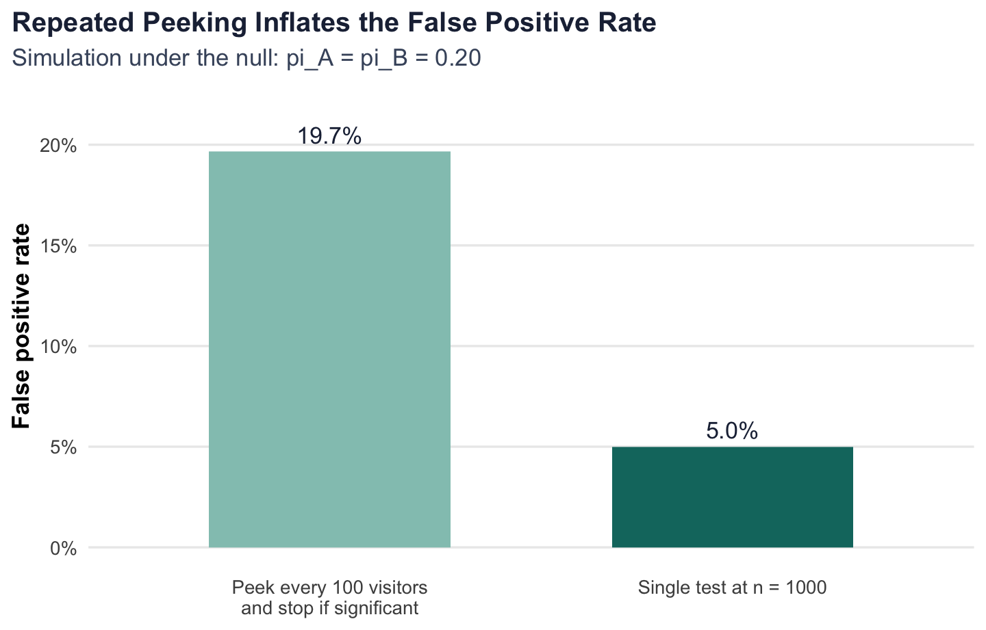
In this simulation, the empirical false positive rate rises to 19.7%, far above the nominal 5% rate of a single planned test. That is the practical problem with peeking: even when there is no real difference between the CTAs, repeated looks at the data make it much easier to convince yourself that you have found a winner.
For real A/B testing, the lesson is simple. If I want valid classical inference, I should commit in advance to a sample size or use a formal sequential-testing framework designed for interim looks. Otherwise, the p-values stop meaning what I think they mean.
Conclusion
This simple CTA experiment shows how a familiar product question maps directly onto the main tools of classical frequentist statistics. The difference in sign-up rates gives a natural estimator, the Law of Large Numbers explains why it stabilizes, the bootstrap and analytical formulas quantify uncertainty, the Central Limit Theorem supports large-sample inference, and regression provides an equivalent and more flexible way to estimate the same effect.
Just as importantly, the peeking example shows that good statistical practice is not only about formulas. Experimental design decisions shape what our p-values and confidence intervals actually mean. In that sense, A/B testing is not just a technical exercise in comparing two buttons or two phrases. It is a disciplined way of learning from data while being honest about uncertainty.