Poisson Regression and Maximum Likelihood Estimation
A case study of Blueprinty’s software and patent awards
Estimating whether Blueprinty’s patent-application software is associated with more awarded patents using maximum likelihood and Poisson regression.
Introduction
Blueprinty is a small software company focused on a very specific workflow: helping engineering firms prepare blueprints for patent applications to the U.S. Patent Office. The marketing question is direct and tempting: can Blueprinty credibly say that firms using its software get more patents approved?
The cleanest way to answer that question would be to observe the same firms before and after adopting Blueprinty, or even better, to randomly assign comparable firms to use or not use the software. That is not the dataset we have. Instead, Blueprinty collected cross-sectional data on 1500 mature engineering firms. For each firm we observe the number of patents awarded over the last five years, the firm’s region, its age since incorporation, and whether it is a Blueprinty customer.
That makes the claim non-trivial. Blueprinty customers were not selected at random. If customers have more patents, the difference might reflect the software, but it might also reflect that customers tend to be older, concentrated in certain regions, better funded, or more patent-oriented in ways we cannot fully observe. The job of the model is to compare customers and non-customers while accounting for the differences we can measure.
TipThe Question I Want The Model To Answer
The raw comparison is useful, but it is not enough for a marketing claim. The better question is:
Among firms with similar age and regional profiles, are Blueprinty customers expected to receive more patents?
Exploring the Data
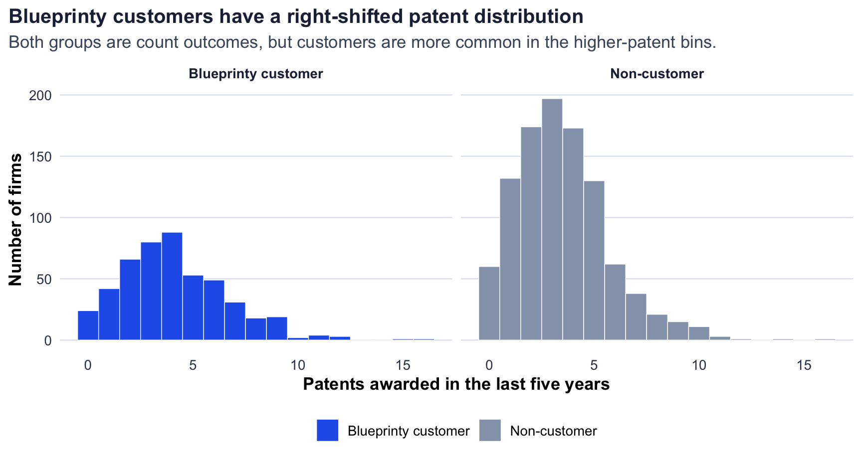
The first look is promising for Blueprinty. Customers average 4.13 patents over the five-year window, while non-customers average 3.47. The raw gap is therefore about 0.66 patents, or a 19.0% higher average patent count for customers.
The distributions overlap heavily, which is important: this is not a case where every customer outperforms every non-customer. Still, the customer distribution is shifted to the right. Customers appear more frequently in the middle and upper patent-count bins, suggesting a positive association before any adjustment.
| Patent Counts by Customer Status | |||
| The unadjusted comparison favors Blueprinty, but it is not yet a causal estimate. | |||
| Group | Firms | Mean patents | Median patents |
|---|---|---|---|
| Blueprinty customer | 481 | 4.13 | 4 |
| Non-customer | 1019 | 3.47 | 3 |
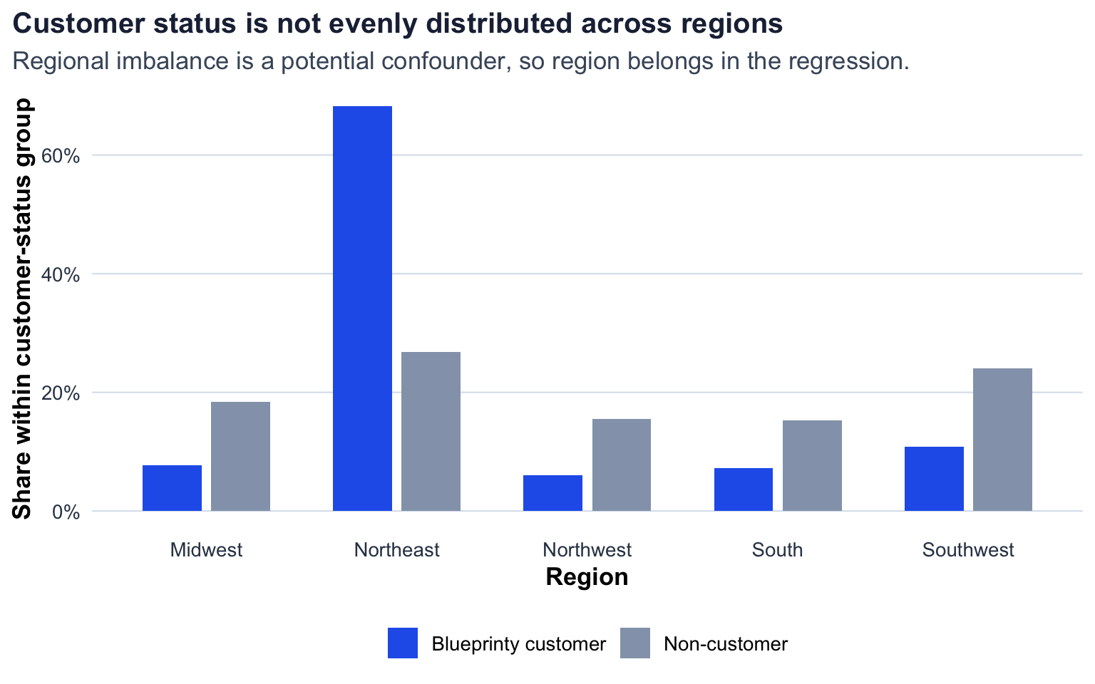
The problem is that customer status is also related to region. Blueprinty’s customer base is especially concentrated in the Northeast: 68% of customers are in the Northeast, compared with 27% of non-customers. If patenting opportunities, industry mix, legal support, or regional innovation ecosystems differ by region, then a raw customer/non-customer comparison partially mixes the software question with a geography question.
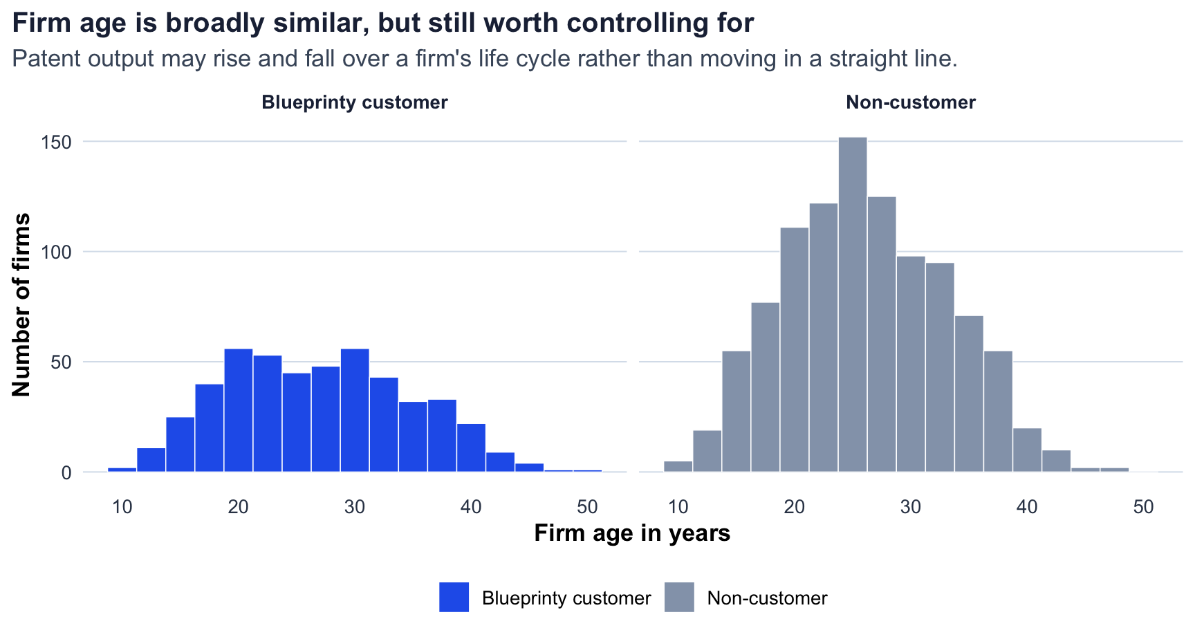
Age is more balanced than region, but it still matters analytically. Customers average 26.90 years old and non-customers average 26.10 years old. Since older firms may have more established R&D processes, deeper patent portfolios, or more legal experience, age should also be held fixed when estimating the customer association.
A Simple Poisson Model via Maximum Likelihood
Patent counts are non-negative integers, so a Normal model is not the most natural starting point. A Normal distribution can put probability on negative patent counts and treats the outcome as continuous. The Poisson distribution is designed for count data, making it a useful first model for the number of patents awarded to a firm.
The maximum likelihood idea is simple in words: try possible values of the unknown rate, calculate how plausible the observed data would be under each one, and keep the value that makes the data most plausible. For a count model, that unknown rate is (), the expected number of patents.
For a single firm, suppose:
\[ Y \sim \text{Poisson}(\lambda) \]
Then the probability of observing a patent count (Y) is:
\[ f(Y|\lambda) = \frac{e^{-\lambda}\lambda^Y}{Y!} \]
If the observations are independent and identically distributed, the joint likelihood for (n) firms is the product of the individual probabilities:
\[ L(\lambda | Y_1,\dots,Y_n) = \prod_{i=1}^{n} \frac{e^{-\lambda}\lambda^{Y_i}}{Y_i!} \]
Taking logs turns the product into a sum:
\[ \ell(\lambda) = \sum_{i=1}^{n} \log\left(\frac{e^{-\lambda}\lambda^{Y_i}}{Y_i!}\right) \]
Using log rules, this simplifies to:
\[ \ell(\lambda) = \sum_{i=1}^{n} \left[-\lambda + Y_i\log(\lambda) - \log(Y_i!)\right] \]
The maximum likelihood estimate is the value of () that makes the observed patent counts most likely.
poisson_loglikelihood <- function(lambda, Y) {
  if (lambda <= 0) {
    return(-Inf)
  }

  sum(Y * log(lambda) - lambda - lgamma(Y + 1))
}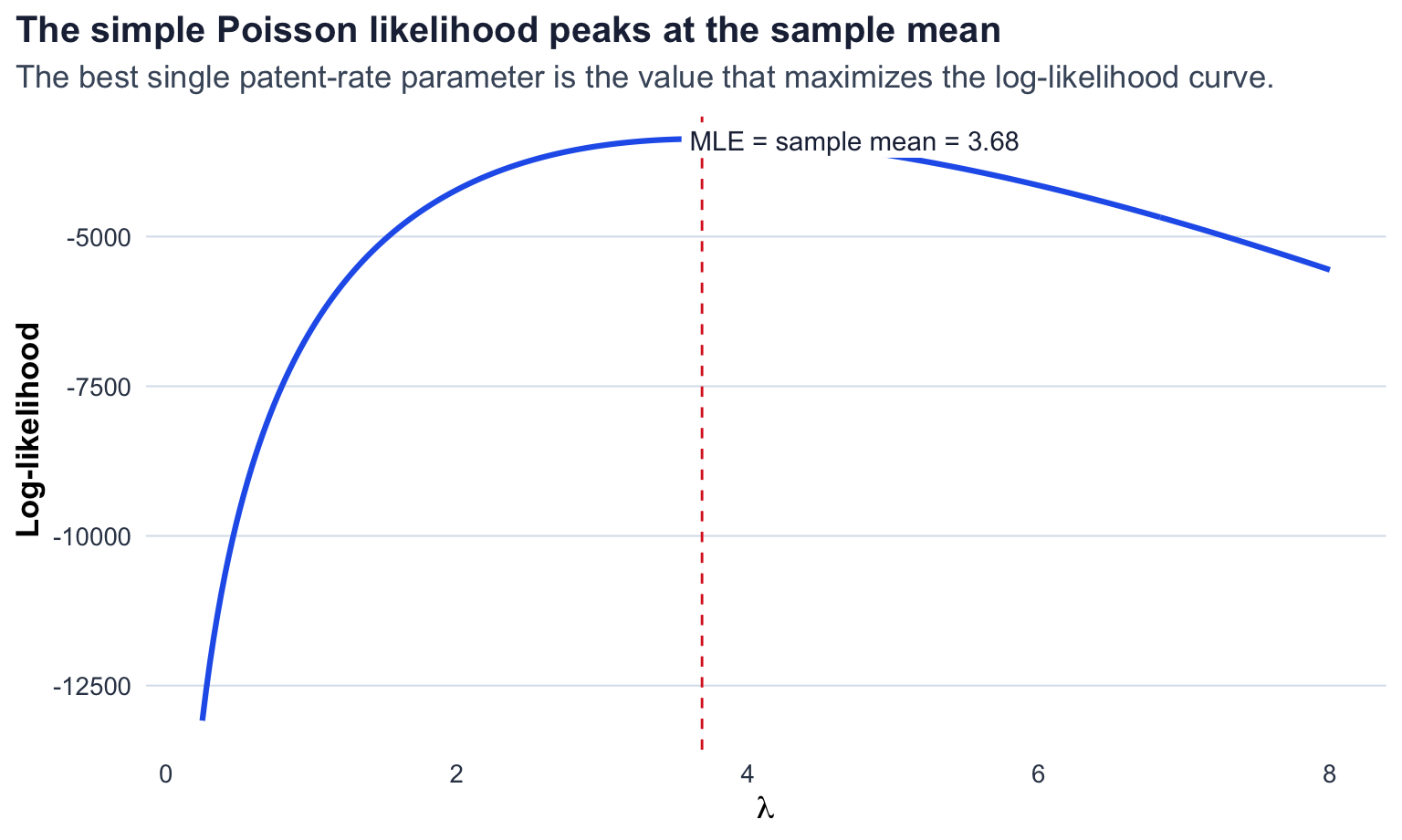
Visually, the curve peaks around 3.68 patents. That peak is the MLE. Values much lower or much higher than the observed average make the full set of patent counts less plausible. The numerical optimizer gives ( =) 3.68, which matches the sample mean of 3.68.
This also follows directly from the derivative. Starting from:
\[ \ell(\lambda)=\sum_{i=1}^{n}\left[-\lambda+Y_i\log(\lambda)-\log(Y_i!)\right] \]
Differentiate with respect to ():
\[ \frac{\partial \ell}{\partial \lambda} =\sum_{i=1}^{n}\left[-1+\frac{Y_i}{\lambda}\right] = -n+\frac{\sum_{i=1}^{n}Y_i}{\lambda} \]
Setting this equal to zero gives:
\[ \hat{\lambda}_{MLE}=\frac{1}{n}\sum_{i=1}^{n}Y_i=\bar{Y} \]
That result feels right: in a Poisson model, () is the expected count, so the best one-parameter estimate is the observed average count. The regression version below uses the same logic, but instead of estimating one shared (), it estimates a different expected count for each firm.
Poisson Regression
The simple model assumes every firm has the same patent rate. That is too restrictive for Blueprinty’s business question. Firms differ by age, region, and customer status, so I next estimate a Poisson regression:
\[ Y_i \sim \text{Poisson}(\lambda_i) \qquad \text{where} \qquad \lambda_i = \exp(X_i'\beta) \]
The exponential link is essential because (_i) must be positive, while a linear index (X_i’) can be any real number. The model lets expected patent counts vary across firms while keeping the prediction on the correct count-data scale.
The covariate matrix includes an intercept, firm age, age squared, region indicators, and the customer indicator. Age squared allows patent productivity to follow a curved life-cycle pattern rather than forcing a straight-line age effect. One region is automatically dropped by model.matrix() because including every region plus an intercept would create perfect collinearity.
poisson_regression_loglikelihood <- function(beta, Y, X) {
  eta <- as.vector(X %*% beta)
  lambda <- exp(eta)

  sum(Y * eta - lambda - lgamma(Y + 1))
}

Y <- blueprinty$patents
X <- model.matrix(~ age + I(age^2) + region + iscustomer, data = blueprinty)

negative_loglikelihood <- function(beta) {
  -poisson_regression_loglikelihood(beta, Y, X)
}

optim_fit <- optim(
  par = rep(0, ncol(X)),
  fn = negative_loglikelihood,
  method = "BFGS",
  hessian = TRUE,
  control = list(
    maxit = 50000,
    reltol = 1e-12,
    parscale = c(1, 0.1, 0.001, rep(1, ncol(X) - 3))
  )
)

beta_hat <- optim_fit$par
names(beta_hat) <- colnames(X)

lambda_hat <- as.vector(exp(X %*% beta_hat))
loglik_hessian <- -t(X) %*% (X * lambda_hat)
optim_se <- sqrt(diag(-solve(loglik_hessian)))

glm_fit <- glm(
  patents ~ age + I(age^2) + region + iscustomer,
  family = poisson,
  data = blueprinty
)

glm_se <- sqrt(diag(vcov(glm_fit)))

coef_plot_data <- tibble(
  term = names(beta_hat),
  estimate = beta_hat,
  se = optim_se
) |>
  filter(term != "(Intercept)") |>
  mutate(
    term = recode(
      term,
      "age" = "Age",
      "I(age^2)" = "Age squared",
      "regionNortheast" = "Northeast",
      "regionNorthwest" = "Northwest",
      "regionSouth" = "South",
      "regionSouthwest" = "Southwest",
      "iscustomer" = "Blueprinty customer"
    ),
    rate_ratio = exp(estimate),
    lower = exp(estimate - 1.96 * se),
    upper = exp(estimate + 1.96 * se),
    term = factor(term, levels = rev(c(
      "Age",
      "Age squared",
      "Northeast",
      "Northwest",
      "South",
      "Southwest",
      "Blueprinty customer"
    )))
)| Poisson Regression Estimates | ||||
| The hand-coded MLE and glm() estimates land on the same answer. | ||||
| Term | MLE coefficient | MLE std. error | GLM coefficient | GLM std. error |
|---|---|---|---|---|
| Intercept | -0.5085 | 0.1832 | -0.5089 | 0.1832 |
| age | 0.1486 | 0.0139 | 0.1486 | 0.0139 |
| Age squared | -0.0030 | 0.0003 | -0.0030 | 0.0003 |
| Region: Northeast | 0.0292 | 0.0436 | 0.0292 | 0.0436 |
| Region: Northwest | -0.0176 | 0.0538 | -0.0176 | 0.0538 |
| Region: South | 0.0565 | 0.0527 | 0.0566 | 0.0527 |
| Region: Southwest | 0.0506 | 0.0472 | 0.0506 | 0.0472 |
| Blueprinty customer | 0.2076 | 0.0309 | 0.2076 | 0.0309 |
The hand-coded MLE and glm() estimates match closely. The small differences are numerical rather than substantive. I asked optim() for the Hessian, and for the standard errors I evaluated the Poisson log-likelihood Hessian at the MLE directly; that is more stable here because the age and age-squared columns live on very different scales.
The customer coefficient is positive: 0.208. In a Poisson regression, coefficients are on the log expected-count scale. Exponentiating the customer coefficient gives 1.231, meaning the model predicts roughly 23.1% more patents for Blueprinty customers than otherwise similar non-customers, holding age and region fixed.
The age pattern is also sensible. The coefficient on age is positive and the coefficient on age squared is negative, which implies expected patent counts rise with age at first but eventually flatten or decline. Region effects are modest in this specification, but including them matters because customer status is not regionally balanced.
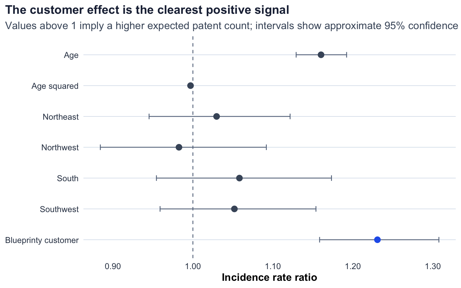
The plot shows the regression in the scale a business reader can interpret. The vertical line at 1 means “no multiplicative change.” The Blueprinty customer estimate sits clearly to the right of that line, while the regional coefficients are much closer to 1.
The Effect of Blueprinty’s Software
Because the Poisson regression is multiplicative, the customer coefficient is not directly an “additional patents” number. To make the result more business-readable, I use two counterfactual prediction datasets:
- (X_0): each firm’s actual age and region, but with
iscustomerset to 0. - (X_1): each firm’s actual age and region, but with
iscustomerset to 1.
The difference between the predicted counts, (_1 - _0), estimates how many additional patents the model associates with Blueprinty customer status for each firm, holding the observed age and region profile fixed.
| Counterfactual Prediction Summary | |
| Same firms, same ages, same regions; only customer status changes. | |
| Scenario | Expected patents |
|---|---|
| All firms treated as non-customers | 3.436 |
| All firms treated as Blueprinty customers | 4.229 |
| Average model-implied difference | 0.793 |
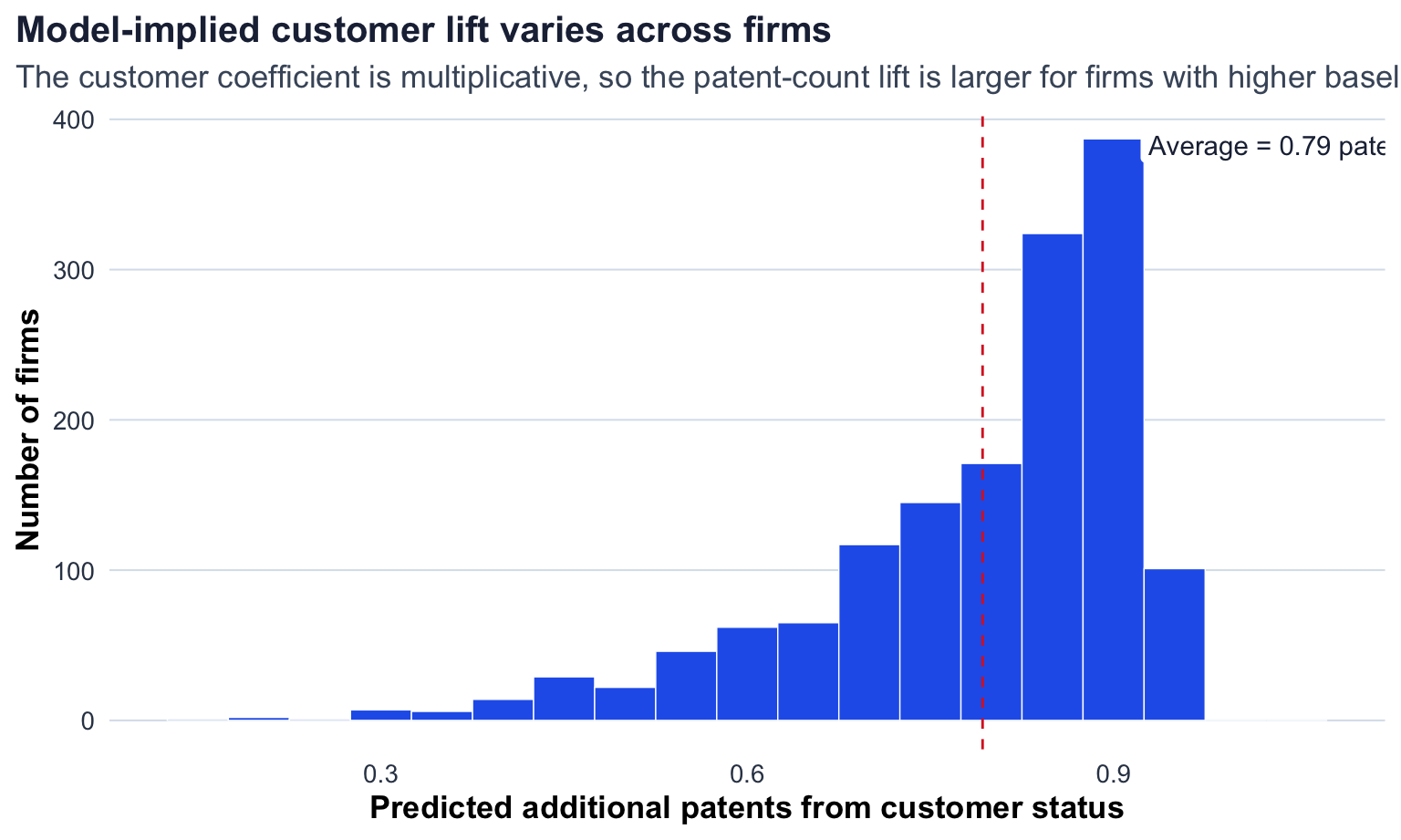
The model estimates that Blueprinty customer status is associated with an average increase of about 0.79 patents over five years, holding each firm’s age and region fixed. That is a meaningful business result: it supports the marketing team’s claim that Blueprinty users are more successful in receiving patent awards.
| What Blueprinty Can Say | |
| Question | Answer |
|---|---|
| What is the raw customer advantage? | Customers average 0.66 more patents over five years. |
| What is the adjusted multiplicative lift? | Customers are predicted to have 23.1% more patents than comparable non-customers. |
| What is the adjusted patent-count lift? | The average counterfactual difference is 0.79 patents over five years. |
| Can we call this definitive causal proof? | No. The result is consistent with Blueprinty's claim, but the data are observational. |
The careful wording is important. This analysis is evidence consistent with Blueprinty’s claim, not definitive causal proof. The data are observational, so unobserved differences may remain. For example, firms that choose Blueprinty may already be more patent-focused, have stronger legal teams, or produce more patentable engineering work. With the available data, the best conclusion is that Blueprinty customers have higher expected patent counts even after controlling for age and region, but a randomized experiment or richer before-and-after data would be needed to make a stronger causal claim.