| MaxDiff Task Structure Check | |||||
| Tasks | 4-item tasks | One best | One worst | Two neutral | All valid? |
|---|---|---|---|---|---|
| 680 | 680 | 680 | 680 | 680 | TRUE |
MaxDiff Analysis of MSBA Class Preferences
Counts, maximum likelihood, and Bayesian MNL estimates
Estimating relative preferences for ten MSBA core classes using Best-Worst Scaling, MNL maximum likelihood, and a Metropolis-Hastings Bayesian model.
Introduction
MaxDiff, also called Best-Worst Scaling, is a survey method for learning relative preferences. Instead of asking people to rate every option on a 1-to-10 scale, it asks them to make trade-offs. On each screen, a respondent sees a small set of items and chooses the one they like most and the one they like least.
That setup is useful here because people often use rating scales differently. One student might call almost everything a 9, while another student saves 9s for rare favorites. MaxDiff pushes respondents to compare the options directly, so the data reveal which classes win when they are placed next to other classes.
In this assignment, the items are the 10 core MSBA classes at UCSD Rady. I estimate class preferences three ways: a simple counts score, a multinomial logit model fit by maximum likelihood, and the same MNL model fit with a Bayesian Metropolis-Hastings sampler. I expect the methods to agree on the top and bottom classes, with more movement in the middle where preferences are closer together.
The Data
The dataset contains 85 respondents. Each respondent completed 15 MaxDiff tasks, each task showed 4 classes, and the study included 10 total classes.
The sanity check passes: every task has exactly one best choice, one worst choice, and two unselected items. The exposure counts are also balanced. Every item was shown either 323 or 595 times, so differences in preference are not being driven by one class appearing much more often than another.
| Exposure by Class | ||
| Item | Class | Times shown |
|---|---|---|
| 1 | MGTA 403 AI Math, Prog., & Analytics (Summer with Nijs) | 332 |
| 2 | MGTA 464 SQL (Summer with Nijs) | 340 |
| 3 | MGTA 451 Marketing/Finance/Operations (Summer with Wilbur/Buti/Shin) | 326 |
| 4 | MGTA 452 Large Data (Fall with Hansen) | 338 |
| 5 | MGTA 453 Business Analytics (Fall with August) | 327 |
| 6 | MGTA 444 Analytics Consulting (Winter with Peterson) | 323 |
| 7 | MGTA 455 Customer Analytics (Winter with Nijs) | 335 |
| 8 | MGTA 454 Capstone Project (Spring with Advisor) | 330 |
| 9 | MGTA 495 Marketing Analytics (Spring with Yavorsky) | 330 |
| 10 | MGTA 457 Biz. Intelligence Systems (Fall with Schibler) | 334 |
| 11 | NA | 595 |
Counts Analysis
The counts analysis is the fastest way to summarize the survey. For each class, I calculate the percentage of appearances where it was selected as best and subtract the percentage of appearances where it was selected as worst:
\[ \text{score}_j = \%\text{best}_j - \%\text{worst}_j \]
A positive score means the class is chosen as best more often than worst. A negative score means the opposite. This method is descriptive and easy to explain, though it does not fully model the choice process.
| Counts Scores by Class | |||||||
| Item | Class | Shown | Best | Worst | % best | % worst | Score |
|---|---|---|---|---|---|---|---|
| 9 | MGTA 495 Marketing Analytics (Spring with Yavorsky) | 330 | 199 | 12 | 60.3% | 3.6% | 0.567 |
| 5 | MGTA 453 Business Analytics (Fall with August) | 327 | 143 | 55 | 43.7% | 16.8% | 0.269 |
| 7 | MGTA 455 Customer Analytics (Winter with Nijs) | 335 | 155 | 71 | 46.3% | 21.2% | 0.251 |
| 11 | NA | 595 | 135 | 0 | 22.7% | 0.0% | 0.227 |
| 4 | MGTA 452 Large Data (Fall with Hansen) | 338 | 122 | 60 | 36.1% | 17.8% | 0.183 |
| 8 | MGTA 454 Capstone Project (Spring with Advisor) | 330 | 124 | 69 | 37.6% | 20.9% | 0.167 |
| 2 | MGTA 464 SQL (Summer with Nijs) | 340 | 111 | 56 | 32.6% | 16.5% | 0.162 |
| 10 | MGTA 457 Biz. Intelligence Systems (Fall with Schibler) | 334 | 74 | 55 | 22.2% | 16.5% | 0.057 |
| 1 | MGTA 403 AI Math, Prog., & Analytics (Summer with Nijs) | 332 | 76 | 90 | 22.9% | 27.1% | -0.042 |
| 3 | MGTA 451 Marketing/Finance/Operations (Summer with Wilbur/Buti/Shin) | 326 | 75 | 101 | 23.0% | 31.0% | -0.080 |
| 6 | MGTA 444 Analytics Consulting (Winter with Peterson) | 323 | 61 | 111 | 18.9% | 34.4% | -0.155 |
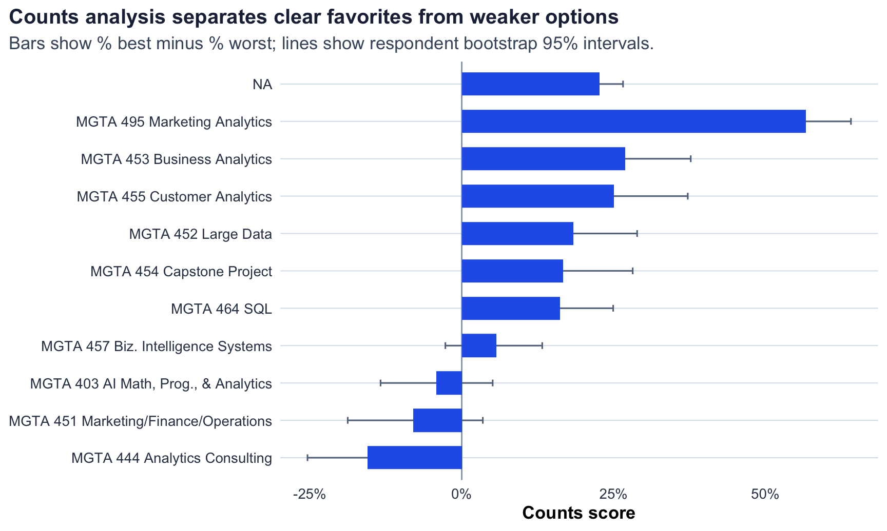
The counts method ranks MGTA 495 Marketing Analytics highest and MGTA 444 Analytics Consulting lowest. The middle of the ranking is closer together, which is exactly where I would expect small sampling variation to change the order.
From MaxDiff Data to MNL Choices
For the MNL model, each task becomes two choice observations. First, the respondent chooses the best class from the four shown. If the shown set is ({a,b,c,d}), the probability of choosing class (b) as best is:
\[ P(\text{best}=b) = \frac{\exp(\beta_b)} {\exp(\beta_a)+\exp(\beta_b)+\exp(\beta_c)+\exp(\beta_d)} \]
Second, after the best class is removed, the respondent chooses the worst class from the remaining three. Since low-utility items are more likely to be chosen as worst, the utilities are flipped:
\[ P(\text{worst}=c \mid \text{best}=b) = \frac{\exp(-\beta_c)} {\exp(-\beta_a)+\exp(-\beta_c)+\exp(-\beta_d)} \]
Only relative utilities are identified. Adding the same constant to every () does not change any soft-max probabilities. I set item 1, MGTA 403, to (_1 = 0), and estimate the other nine utilities relative to that reference class.
MNL via Maximum Likelihood
The log-likelihood sums the best-choice probability and the worst-choice probability over all tasks:
\[ \ell(\boldsymbol{\beta}) = \sum_{\text{tasks}} \left[ \beta_{j_b^*} - \log \sum_{j \in \text{shown}} \exp(\beta_j) - \beta_{j_w^*} - \log \sum_{j \in \text{shown}\setminus\{j_b^*\}} \exp(-\beta_j) \right] \]
I maximized this likelihood with optim() using BFGS and used the inverse negative Hessian for standard errors. To make the estimates easier to read, I also convert utilities into shares of preference:
\[ \hat{s}_j = \frac{\exp(\hat{\beta}_j)}{\sum_{k=1}^{10}\exp(\hat{\beta}_k)} \]
These shares answer a simple hypothetical question: if all 10 classes appeared on one screen, what share of choices would each class receive?
| MNL Maximum Likelihood Estimates | ||||
| Item | Class | MLE beta | SE | Preference share |
|---|---|---|---|---|
| 9 | MGTA 495 Marketing Analytics (Spring with Yavorsky) | 1.630 | 0.146 | 28.4% |
| 5 | MGTA 453 Business Analytics (Fall with August) | 0.744 | 0.142 | 11.7% |
| 7 | MGTA 455 Customer Analytics (Winter with Nijs) | 0.656 | 0.142 | 10.7% |
| 4 | MGTA 452 Large Data (Fall with Hansen) | 0.555 | 0.140 | 9.7% |
| 8 | MGTA 454 Capstone Project (Spring with Advisor) | 0.443 | 0.140 | 8.7% |
| 2 | MGTA 464 SQL (Summer with Nijs) | 0.438 | 0.137 | 8.6% |
| 10 | MGTA 457 Biz. Intelligence Systems (Fall with Schibler) | 0.236 | 0.137 | 7.0% |
| 1 | MGTA 403 AI Math, Prog., & Analytics (Summer with Nijs) | 0.000 | Reference | 5.6% |
| 3 | MGTA 451 Marketing/Finance/Operations (Summer with Wilbur/Buti/Shin) | -0.067 | 0.139 | 5.2% |
| 6 | MGTA 444 Analytics Consulting (Winter with Peterson) | -0.239 | 0.141 | 4.4% |
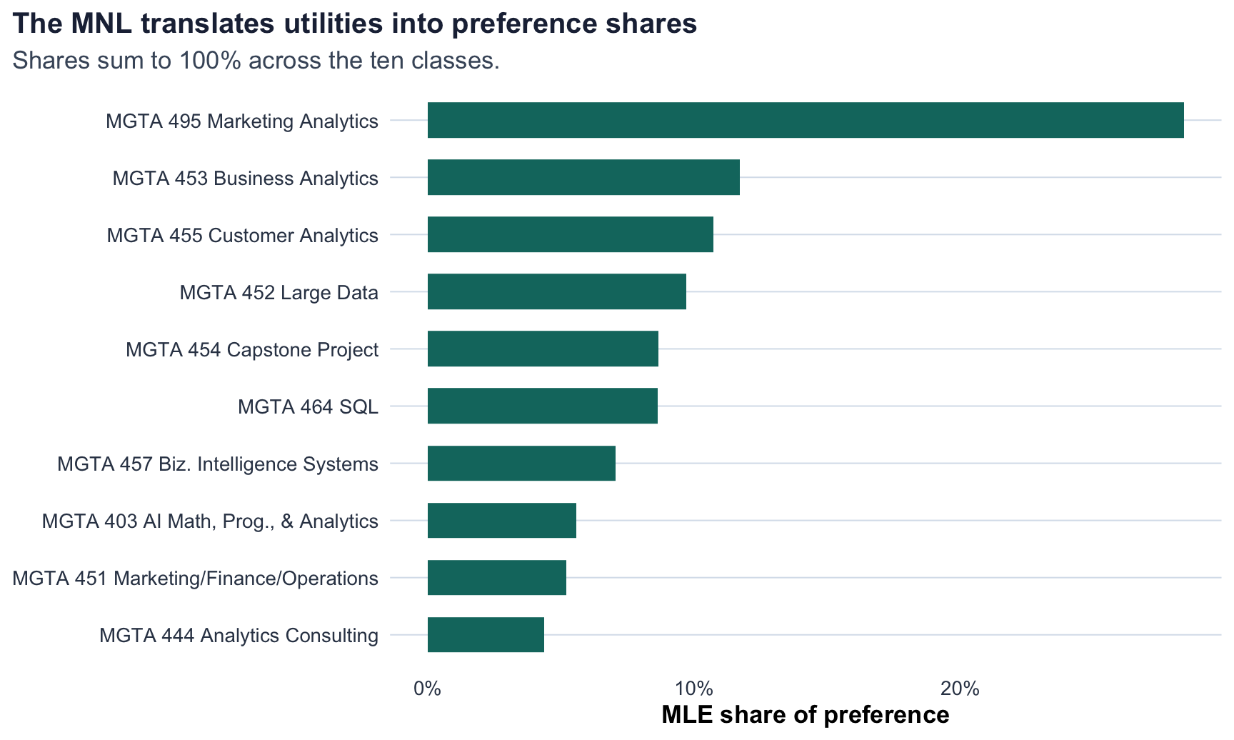
The MLE model ranks MGTA 495 Marketing Analytics first and MGTA 444 Analytics Consulting last. Compared with counts, the broad story is similar, but the MNL uses more structure: it accounts for the specific competitors present in each task and treats not being selected as information.
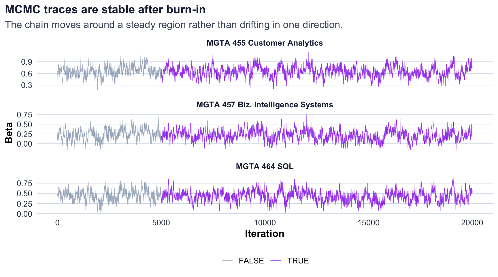
MNL via Bayesian Estimation
The Bayesian model uses the same likelihood, but combines it with a weakly informative Normal prior:
\[ \boldsymbol{\beta} \sim N(\boldsymbol{0}, 10I) \]
I used a random-walk Metropolis-Hastings sampler. The proposal step size was tuned to 0.07, which produced an acceptance rate of 34.9%. I ran 20,000 iterations and discarded the first 5,000 as burn-in.
| Bayesian MNL Estimates | ||||
| Item | Class | Posterior mean beta | 95% credible interval | Posterior mean share |
|---|---|---|---|---|
| 9 | MGTA 495 Marketing Analytics (Spring with Yavorsky) | 1.617 | [1.323, 1.917] | 28.3% |
| 5 | MGTA 453 Business Analytics (Fall with August) | 0.731 | [0.470, 1.018] | 11.7% |
| 7 | MGTA 455 Customer Analytics (Winter with Nijs) | 0.647 | [0.386, 0.916] | 10.8% |
| 4 | MGTA 452 Large Data (Fall with Hansen) | 0.543 | [0.265, 0.812] | 9.7% |
| 2 | MGTA 464 SQL (Summer with Nijs) | 0.431 | [0.167, 0.705] | 8.7% |
| 8 | MGTA 454 Capstone Project (Spring with Advisor) | 0.429 | [0.159, 0.710] | 8.6% |
| 10 | MGTA 457 Biz. Intelligence Systems (Fall with Schibler) | 0.216 | [-0.034, 0.463] | 7.0% |
| 1 | MGTA 403 AI Math, Prog., & Analytics (Summer with Nijs) | 0.000 | [0.000, 0.000] | 5.6% |
| 3 | MGTA 451 Marketing/Finance/Operations (Summer with Wilbur/Buti/Shin) | -0.075 | [-0.341, 0.224] | 5.2% |
| 6 | MGTA 444 Analytics Consulting (Winter with Peterson) | -0.254 | [-0.510, 0.022] | 4.4% |
The Bayesian estimates are very close to the MLE estimates, which is reassuring because the prior is weak and the dataset is fairly large. The main advantage is interpretability of uncertainty: once I have posterior draws, credible intervals for shares are easy to calculate directly.
Comparing the Three Methods
| Side-by-Side Ranking Comparison | |||||||
| Item | Class | Counts score | Counts rank | MLE share | MLE rank | Bayes share | Bayes rank |
|---|---|---|---|---|---|---|---|
| 9 | MGTA 495 Marketing Analytics (Spring with Yavorsky) | 0.567 | 1 | 28.4% | 1 | 28.3% | 1 |
| 5 | MGTA 453 Business Analytics (Fall with August) | 0.269 | 2 | 11.7% | 2 | 11.7% | 2 |
| 7 | MGTA 455 Customer Analytics (Winter with Nijs) | 0.251 | 3 | 10.7% | 3 | 10.8% | 3 |
| 4 | MGTA 452 Large Data (Fall with Hansen) | 0.183 | 5 | 9.7% | 4 | 9.7% | 4 |
| 8 | MGTA 454 Capstone Project (Spring with Advisor) | 0.167 | 6 | 8.7% | 5 | 8.6% | 6 |
| 2 | MGTA 464 SQL (Summer with Nijs) | 0.162 | 7 | 8.6% | 6 | 8.7% | 5 |
| 10 | MGTA 457 Biz. Intelligence Systems (Fall with Schibler) | 0.057 | 8 | 7.0% | 7 | 7.0% | 7 |
| 1 | MGTA 403 AI Math, Prog., & Analytics (Summer with Nijs) | -0.042 | 9 | 5.6% | 8 | 5.6% | 8 |
| 3 | MGTA 451 Marketing/Finance/Operations (Summer with Wilbur/Buti/Shin) | -0.080 | 10 | 5.2% | 9 | 5.2% | 9 |
| 6 | MGTA 444 Analytics Consulting (Winter with Peterson) | -0.155 | 11 | 4.4% | 10 | 4.4% | 10 |
| 11 | NA | 0.227 | 4 | NA | NA | NA | NA |
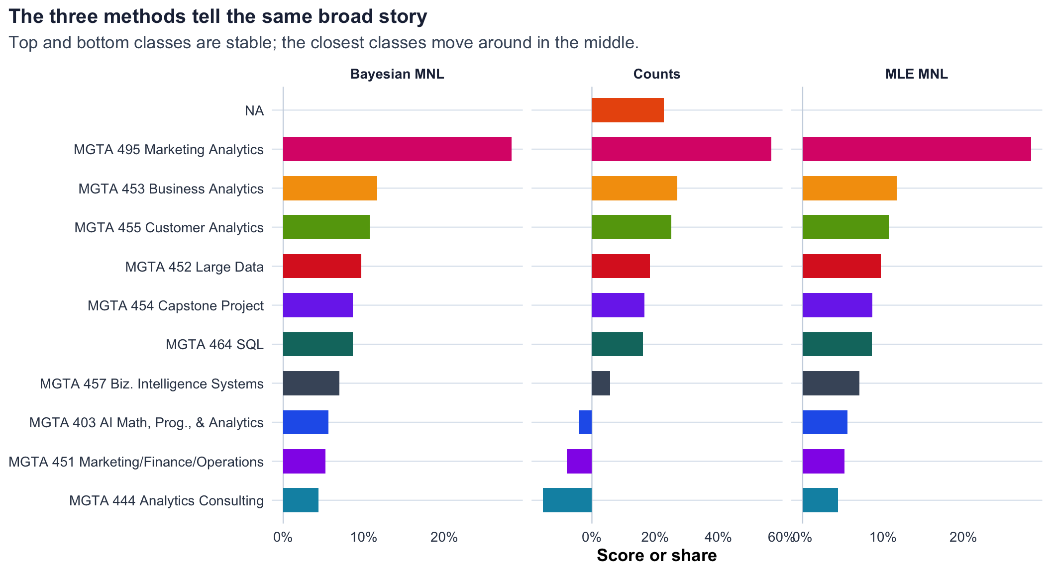
The three methods agree most strongly at the extremes. MGTA 495 Marketing Analytics is the top Bayesian class, and MGTA 444 Analytics Consulting is the bottom Bayesian class; these line up closely with the counts and MLE results. The disagreements are mostly in the middle, where several classes have similar scores and small differences can flip the order.
Counts are useful for a quick dashboard because the score is transparent. MLE adds a formal choice model and produces standard errors for the estimated utilities. Bayes adds an even more flexible uncertainty workflow, especially for derived quantities like preference shares.
Discussion
Substantively, the survey suggests that students have clearer enthusiasm for the top analytics and systems-oriented classes than for the lower-ranked required classes. I would be careful not to overstate the exact middle ranking, because the uncertainty bands overlap for several options.
For a non-technical audience, I would show the counts result first because it is intuitive: how often did each class win versus lose when shown? For a formal report, I would use the MLE MNL estimates because they match the structure of the MaxDiff task. For planning simulations or future model extensions, I would prefer the Bayesian version because posterior draws make uncertainty on any quantity easier to summarize.
The biggest caveat is external validity. These results come from a self-selected sample of MSBA students, and preferences may depend on students’ prior work experience, current quarter, instructors, and how the course names were presented. If I had more time, I would estimate individual-level preferences or segment students by background to see whether the overall ranking hides different taste groups.